Four months ago I was doing research in astrophysics in a Spanish institution and since then I made a change in my career moving to work in Finland. From October 2018 I am working at Boogie Software inside the Artificial Intelligence Team. During the last months, our team has been working with bank data to study the information that can be extracted from it. We are making developments in data synthesis using Deep Learning and customer profiling (please find more information in Boogie AI).
In this post I describe a possible use of bank data. The objective is to make the profile of the client according to the transaction history and predict the success of a potential loan. The selected bank data is from a real Czech bank. It was released anonymized in 1999 and is one of the largest open bank data sets. It contains around 1 million transactions for 4500 accounts. It also provides information about the client products, as loans or credit cards, and other demographic information such as the age and gender of the client, or data about the client’s district.
In this study the goal is to predict how well a client will carry out with the future payments of a loan. In the data there is information about the status of payments for each given loan. The payment status is divided into four categories. The categories describe if the contract is finished or running and if the client has complied with all the monthly payments or if he/she is in default. For this exercise, I divided the loans into two classes depending only on the payment status. The “on schedule” class means that the loan is running or has finished without problems. The “in default” class means that the client has been in default for some months.
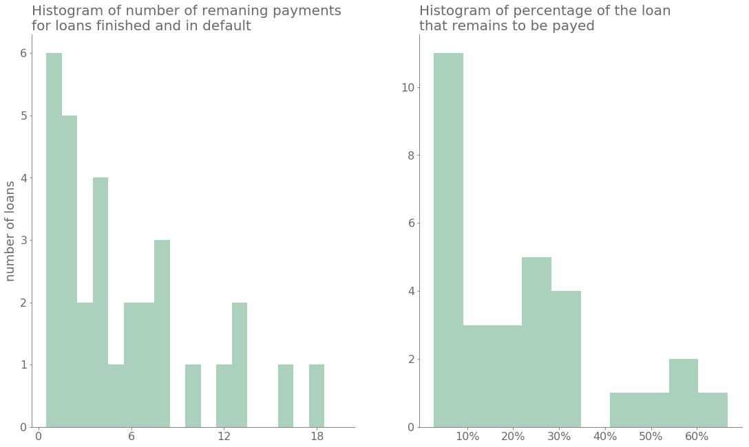
It is worth mentioning that, although some loans are classified as “in default”, often the client has continued making payments. Often, even at the end of the contract, the balance in the account associated with the loan is positive. For example, the following figure shows the number of outstanding payments and the percentage of the loan that remains unpaid. The figure shows how for the “in default” loans the client actually paid a large part of them. In most cases, the client’s balance is in good shape to pay the remaining amounts.
Generating the feature vector
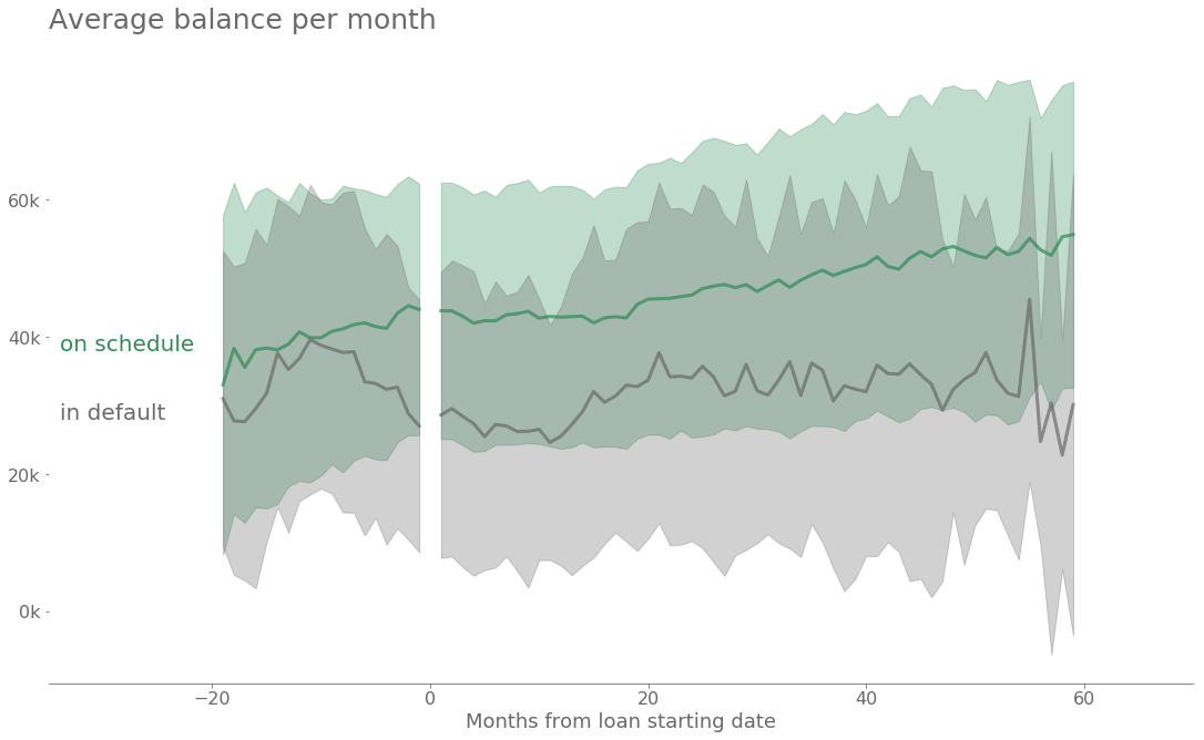
The exercise here is to classify each loan as “on schedule” or “in default” using a feature vector for each client. To generate the features, one has to use the information available before each loan started. For this purpose, monthly averaged properties are computed for each account associated with a loan. Some of these properties are, for example, the average, minimum and maximum balance, the number of incoming and outgoing transactions and some statistics on the associated amounts. Finally, these average properties are referred to the start date of each loan. The following graph shows the average monthly balance stacked for all the clients with loans. The shaded areas in the figure represents the uncertainty. One can see the difference in the loans that go into default.

The monthly aggregated values for the three months before the loan started are used in the final feature vector. Other information is also used, as for example, information relative to the loan itself, the client products, and demographic information.
Predicting loan potential risk
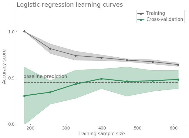
First, it is necessary to select the metric and a simple prediction as baseline. I choose to use the accuracy defined as (correct predictions)/(total sample size). One should note that the number of loans is actually very low. There are only 682 loans and only 76 of them are “in default”. Under these circumstances a good baseline model is to predict that all loans are “on schedule”, which yield a good accuracy score of 0.89. It’s fair to assume that this would be due to the bank using their own tools for selecting which amount of loan it grants to which client, and also because of the client’s commitment to pay back.
 In a first approximation it is good to see the potential of some basic classifiers like Logistic Regression or Naive Bayes. At is is shown in the next figure one can get slight better results than the baseline model.
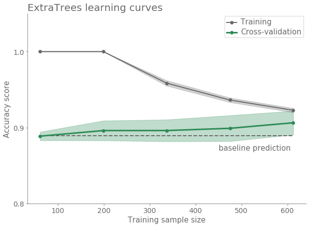
Classifiers based on decision trees bagging produce better results as shown in the following figure.
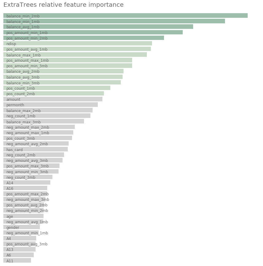
Also an advantage of the models based on decision trees is that they are able to rank the feature importance. The following figure shows which features play a significant role in the prediction. One can see how the analysis done on the client transaction history allows to improve the prediction. One could assume that the balance in the account before granting the loan is an important feature. However, one also understands that often someone needs a loan when the balance is not very high.
Rank the probability of loan success
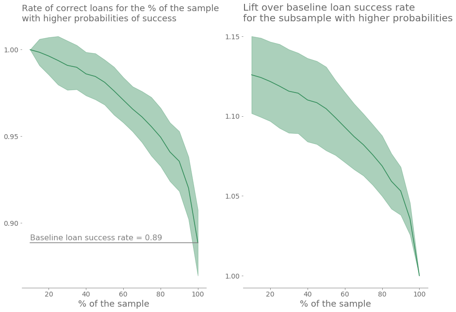
Finally, some classifiers provide a probability for an item to be in a class. We can use these probabilities to rank the loans. In this exercise, a random forest classifier is used to rank the loans using the probability of success. The following figures show the loan success rate for the percentage of the sample that is most likely to be “on schedule” according to the classifier. To produce the curves, the model is trained several times with different random subsets of the loans and the predictions are analyzed on the complementary data. The figures show the average for all the iterations and its standard deviation.
Final remarks
In this article, I used one of the largest open bank data sets to make predictions about how well a client will deal with future loan payments. A similar project could be done (surely it is being done) with real data. The information from these studies will be useful for both the bank and the client. This kind of analysis can be used to adjust the length of the loan and the payments to make them more affordable for the client during the loan period.
Some questions can be raised about the current exercise. On the features side, it is possible that the account has a specific purpose. Also, is possible that the clients have other accounts for other purposes or in other banks. All this information should be aggregated in the feature vector. On the data side, there is a selection of the clients and the loans, so the results are biased towards “on schedule” loans. In fact, even the loans classified as “in default” have been returned mostly, and in the rest, often the clients seem able to complete the payments. This could suggest a tight selection of the clients granted with a loan.
If you find this topic interesting, please find more info about our
AI team offering and do not hesitate to drop a line if you want to discuss more.
References
- Boogie Software Oy is a private Finnish company headquartered in Oulu, Finland. Our unique company profile builds upon top level software competence, entrepreneurial spirit and humane work ethics. The key to our success is close co-operation with the most demanding customers, understanding their business and providing accurate software solutions for complex problems.
- The open bank data used in the article can be found in the following link https://sorry.vse.cz/~berka/challenge/
- A more detailed analysis with additional figures in Jupyter notebooks is available in the following github repository explore-financial-data.
- The analysis has been done using numpy, pandas and scikit-learn Python libraries. The figures have been generated using matplotlib and seaborn libraries.


 In a first approximation it is good to see the potential of some basic classifiers like Logistic Regression or Naive Bayes. At is is shown in the next figure one can get slight better results than the baseline model.