
Predicting Stock Returns with a Neural Network

I spent the summer of 2019 as a Data Analyst trainee at Boogie Software. Part of my work was to implement a small project utilizing neural networks to solve an interesting problem of my own choosing. I have experience in portfolio performance analysis, so I immediately thought of stock market data. More precisely, predicting stock returns with neural networks. Boogie Software has strong expertise in financial technology, so the topic fits nicely to the company profile and the whole AI team was eager to contribute to the work.
Predicting future stock returns has always been a popular topic. Reasonable estimates of expected returns are useful in many financial asset pricing models. Most investors would like to be able to pick the future winning stocks into their portfolio. Predicting stock returns is not easy, but the development of machine learning models provides new possibilities in the field of empirical asset pricing.
In this work, we use an artificial neural network model to predict future stock returns. We also construct investment portfolios based on the predictions. We then compare the performance of the portfolios to the overall stock market. As a difference to many academic papers exploring this topic, we use publicly available data.
Predictive models
Multilayer perceptron (MLP)
We study the performance of a basic feed forward artificial neural network, the multilayer perceptron. We use a simple network with one hidden layer that consists of 32 nodes. Nonlinearity of the network is achieved by using the leaky ReLU activation function. The network is trained using the Adam optimization algorithm, which is an extension to the stochastic gradient descent method. Mean squared prediction error is used as the objective function.
Linear model (OLS)
As a reference model, we use the linear regression model. The linear model is computationally efficient, because the coefficients of the model can be analytically determined by using the ordinary least squares (OLS) method.
Data and methodology
We use price and trading volume data for U.S. stocks traded in the NYSE and NASDAQ. The data set covers 22 years starting from April 1997 and ending on March 2019. The number of stocks starts from 1590 and increases to 4568 by the end of the period. Note that this data set suffers from survival bias as it does not contain historical data for companies that have exited the market during the period. Links to the data sources can be found from the References section below.
We limit our analysis to the top 500 stocks based on the average dollar trading volume during the previous year. The following graph shows the cumulative total return of an equally weighted (EW) portfolio using our top 500 stock selections compared to the S&P 500 index. The correlation between the EW portfolio and the S&P 500 index is 0.94. While not exactly the same thing, this method mimics investing to the S&P 500 index quite well. In the analysis below, the EW portfolio is used to represent the market portfolio.
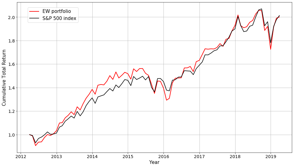 |
| Cumulative total return of the EW portfolio and the S&P 500 index. |
The response variable that we are trying to predict is the excess return over the risk free rate (U.S. Treasury Bill yield) for each stock. W The predictors include e.g. beta, return volatility, illiquidity and momentum return. We also use six macroeconomic variables as predictors including several variables computed from interest rates as well as stock market wide dividend to price and earnings to price ratios. We lag the variables when needed to avoid
We divide the available period of data into ten years of training data and five years of validation data. The training data is used to train the MLP model. The validation data is used for early stopping of training to avoid overfitting the model. We also utilize dropout and L1 penalization of the weight parameters as additional regularization methods for the MLP model. The OLS model does not require the use of validation data, so we use both training and validation data to fit the model.
The last seven years of the data set are reserved for out-of-sample testing. In out-of sample testing the models are refit once every year using monthly data from the preceding training and validation periods. The models are then used to predict next month returns using the previous month predictor variables until the next refit.
Prediction results
We measure the predicting power of the models by computing the out-of-sample coefficient of determination (R2) using the predicted and true excess returns from the seven year testing period. The results are presented in the table below.
| Model | R2 |
|---|---|
| MLP | 3.07 % |
| OLS | 0.05 % |
The R2 metric can be interpreted so that 3.07% of the total variance in stock excess returns is predictable by the MLP model. The OLS model seems to lack any real predicting power. Based on these results it is not feasible to try to predict the future returns of a single company using these models.
Portfolio performance
For portfolio performance testing, we sort the 500 stocks into ten portfolios each month based on their predicted excess returns for the next month. Portfolio HI contains the 50 stocks with the highest predicted returns. Portfolio LO contains the 50 stocks with the lowest predicted returns. The graph below shows the cumulative total returns of the HI and LO portfolios for each model compared to the EW portfolio that contains all 500 stocks.
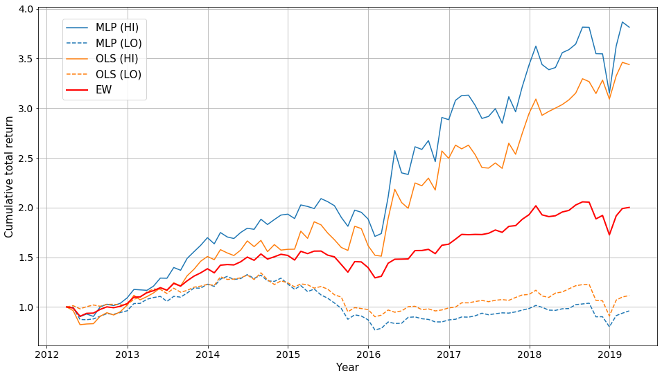 |
| Cumulative total return of the portfolios. |
There is clear separation between the highest and lowest ranked portfolios, which indicates that both models are able to separate good performers from the poor ones. Furthermore, the HI portfolios outperform the EW portfolio for both models. Annualized portfolio performance metrics are shown in the following table (alpha and beta values have been computed against the EW portfolio).
| Metric | MLP (HI) | MLP (LO) | OLS (HI) | OLS (LO) | EW |
|---|---|---|---|---|---|
| Mean excess return | 0.209 | 0.001 | 0.196 | 0.021 | 0.102 |
| Volatility | 0.216 | 0.153 | 0.222 | 0.147 | 0.129 |
| Sharpe ratio | 0.97 | 0.01 | 0.88 | 0.14 | 0.79 |
| Maximum drawdown | 0.182 | 0.420 | 0.186 | 0.329 | 0.173 |
| Turnover (monthly) | 121% | 129% | 115% | 109% | 7.6% |
| Alpha | 0.066 | -0.105 | 0.053 | -0.073 | N/A |
| Alpha t-stat | 1.43 | -3.60 | 1.04 | -2.10 | N/A |
| Beta | 1.40 | 1.04 | 1.39 | 0.92 | 1.00 |
The HI portfolios have much higher volatility (standard deviation of returns) than the EW portfolio. However, due to their high mean returns they have higher risk-adjusted returns (Sharpe ratios) than the EW portfolio. The lowest ranked portfolios show statistically significant negative alphas. The highest ranked portfolios have strong positive alphas, but they are not statistically significant.
One potential problem of implementing these portfolios in practice is high turnover. Rebalancing the portfolios requires trading the whole value of the portfolio each month. The strong mean returns allow for high trading costs, however. For example, the MLP (HI) portfolio maintains the excess return advantage compared to the EW portfolio up to trading costs of 0.8%.
The risk conscious investor is probably more interested in the risk-adjusted returns than in the absolute returns. The Sharpe ratios of the HI portfolios as a function of trading costs in basis points (one hundredth of a percent) are shown in the graph below.
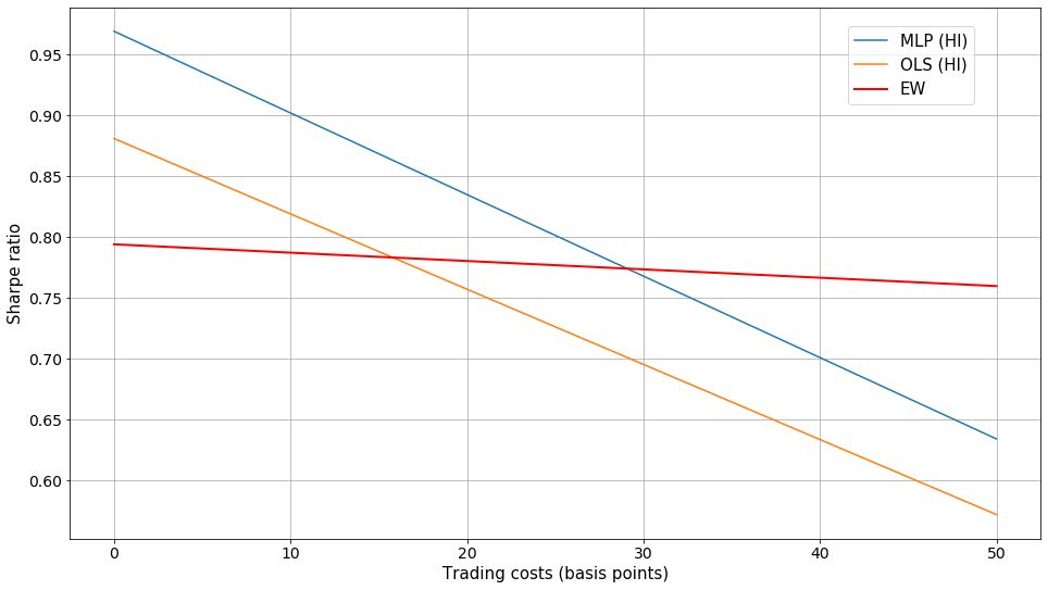 |
| The effect of trading costs to the Sharpe ratio of the portfolios. |
The MLP (HI) portfolio holds the Sharpe ratio advantage compared to the EW portfolio up to trading costs of 29 basis points (0.29%). This is a realistic cost level for the investor who is willing to actively buy and sell on average 60 stocks each month. However, it should be noted that S&P 500 index ETFs performed even better during the test period. Mean excess return of a typical ETF was 0.121 with a volatility of just 0.109 yielding a Sharpe ratio of 1.11 with zero trading costs after the initial investment.
Concluding remarks
The results presented above show that the neural network model is not able to produce very accurate predictions from the noisy stock market data for a single company. It performs better than the linear model, however. Both models have predicting power when stocks are sorted into portfolios. Investing into stocks with high predicted returns can produce higher returns than the average market if the investor is willing to tolerate risk and higher transaction costs.
In addition to the MLP, we have also studied other machine learning models in the context of predicting stock returns. For example, the long short-term memory (LSTM) recurrent neural network is able to process sequences of data. It shows promising results that challenge the performance of the MLP model.
References
- Boogie Software Oy is a private Finnish company headquartered in Oulu, Finland. Our unique company profile builds upon top level software competence, entrepreneurial spirit and humane work ethics. The key to our success is close co-operation with the most demanding customers, understanding their business and providing accurate software solutions for complex problems.
- The methodology used in this work is inspired by the paper Empirical Asset Pricing via Machine Learning by Gu, Kelly and Xiu (2019).
- For stock data, a subset of the kaggle dataset AMEX, NYSE, and NASDAQ stocks histories was used with some additional downloads from Yahoo Finance. Interest rate data was downloaded from FRED (Federal Reserve Economic Data). Market wide D/P and E/P ratios are from Online Data by Robert Shiller.
- The analysis was implemented with Python using numpy, pandas, keras, tensorflow and scikit-learn libraries. The graphs have been created with matplotlib.