In our company we have developed a system and done some research on methodologies to synthesize tabular data and specially customer accounts bank transactions. Our current solution is based on deep neural networks, and have three main components, which use techniques as Generative Adversarial Networks or Long Short Term Memory cells. The solution can be used either to synthesize tabular data considering the rows (transactions) as independent (see as reference our previous blog post on the topic), or to synthesize series of transactions. In the first case, the model can generate data that reproduce the histograms of the individual columns and relationship between them. In the second case, the temporal aspects must also be considered.
In this post I explain an exercise aimed to synthesize complete series of transactions using a single model. For introduction on synthetic data utility in various scenarios see our previous blog posts (see references).
Bank transaction data set
For obvious reasons there are not many publicly available bank transaction data sets. We have been working before with data from a real Czech bank that was released anonymized in 1999. This data set is one of the largest and most complete open bank data sets available online.
The objective of this project was to train a single Deep Learning model capable of synthesizing new series of transactions with properties similar to those of the training data. In this exercise the following columns were considered:
- transaction type. Defined by three different columns: type: indicates mainly if it is a debit or credit transaction and contains categorical values with three potential values, operation: categorical column with five values, and k-symbol: categorical with eight values. Both operation and k-symbol contain missing values that were treated as an additional category. All the categorical columns were one-hot encoded.
- amount. Positive real number. During pre-processing it was transformed into logarithmic scale and scaled in the range [-1, 1].
- balance. Real number. As amount was transformed into logarithmic scale and scaled in the range [-1, 1].
-
date. Date object with resolution of one day indicating when each transaction takes place. In this exercise the date was encoded during pre-processing using the following strategy. Extra transactions types that mark the start of a new month were inserted into the series (these additional entries are not associated with any real transaction). The part of the date object containing the day of the month of each transaction was treated as a float number and scaled in [-1, 1] range. The date was reconstructed during post-processing from a given start date, the marks indicating the beginning of a new month, and the day of the month associated with each synthetic transaction.
Model architecture
Working with Deep Learning models for synthesizing tabular data, we have learned that Generative Adversarial Networks are the main path to focus on. Our previous experience also indicates that training such models is complex, and that using Wasserstein loss (WGAN-GP) ease the job. Finally, another good potential ingredient for a model capable of producing series of transactions is the recurrent capacity.
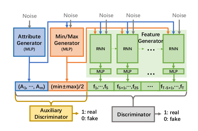
There is extensive research in the field of synthetic data when referring to images. Nevertheless, we have not found so many approaches that deal with tabular data, especially for transactions or time series. Last December, I found an article that describes an architecture that have all the ingredients described above (
Zinan Lin et al 2019
).The article describes the DoppelGANger software and demonstrates that it works well for time series data. DoppelGANger is implemented using Tensorflow. Its architecture is shown in the following figure that I borrowed from the article. The main component of the generator is a recurrent neural network with LSTM cells. An MLP is attached to the RNN to produce the output of each column in the time series part of the output. The model has the possibility of synthesizing several steps of the time series for each step of the RNN. However, in this exercise only one transaction is produced for each step of the RNN.
To be explicit, in our case the ficontains a vector with the encoded information of a transaction. {f1,..,fT} is the complete set of transactions of an account sorted in temporal order. The article also describe the objects that DoppelGANger takes as input data. Each time series can have associated metadata that is first synthesized by the Attribute Generator. I took advantage of this possibility and used the Attribute Generator to include some global properties of each account (the minimum, maximum, mean and standard deviation of the amount and balance, and which types of transactions are used by the account).
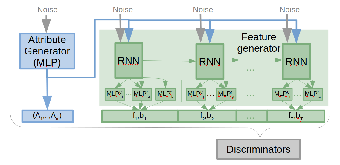
The first results were promising, so I decided to spend some time changing the architecture a bit. With respect to the generator part, the balance in each step of the RNN can be calculated directly (all but the first balance of each series) from the previous balance and the current synthesized amount. Therefore, a modification was made to directly compute the balance instead of synthesizing it using the Feature Generator. Another change was related to the high correlation between the transaction type and the amount. A modification allows to synthesize first the categorical columns and concatenate the result into the MLP that synthesize the amount. The modified architecture is shown in the next figure.

On the discriminator side, I have included new discriminators into the model. I thought that having a discriminator that sees only part of the transactions, or even individual transactions can improve the correlations between the columns. Therefore a new discriminator can be used that look into a few steps of each series (randomly selected from the real and synthetic series on each batch). In order to improve the sequence of transaction types, another discriminator was included that analyzes the transaction type sequencing. This discriminator sees the part of the vector that defines the transaction type along the entire sequence. One can configure whether or not each discriminator is used and weigh its contribution to the loss, so a few different configurations were tested. The results are based on a model trained during 24 hours in the Google Cloud using a NVIDIA Tesla P100 GPU.
Results
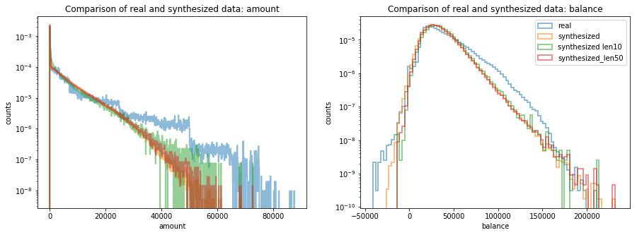
To evaluate how well the model performs, I synthesized 20000 series (accounts) with 150 transactions, and compared the histograms of individual categorical and numerical columns, the correlation between them, and also different temporal aspects of the transactions.
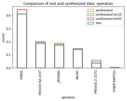
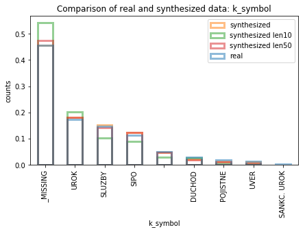
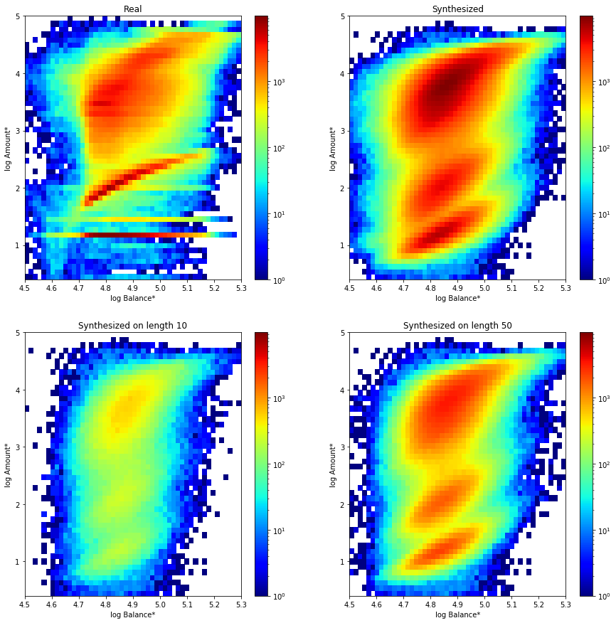
The figures on the right side show the density histograms of the operation and k_symbol categorical columns. It can be seen that the model is quite good in capturing the rate of transactions of each type, although examples of the less represented categories are not as successfully generated. The figure also shows how the values are quite constant for different lengths of the series (histograms with the first 10 and 50 transactions of each account).
The following two figures show the histograms of the two numerical columns (amount and balance). Again, the results are good, however, a slight bias can be observed that prevents large amounts as the series progresses. I suppose that this is caused by the fact that the network can only act on the amount in order control the balance values and large amount values are more prone to cause tails in the low and high balance ends.
The next figure shows the correlation among the amount and balance. It must be said that many of the features in the figure are produced by the tied relation between the amount and the type of transaction. This means that network has learned the correct amount range for each type. In any case, there are also correlations inside each transaction type that are reproduced. On the other hand, with the current parameters, the network cannot synthesize properly constant low amounts that are independent of the balance for certain types. Although the magnitude of the operation is well captured also in this case.
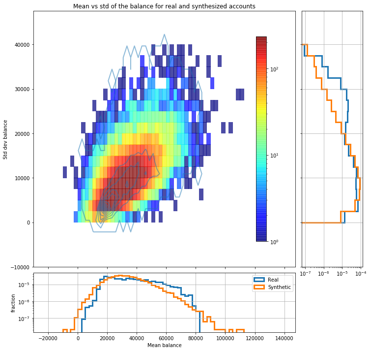
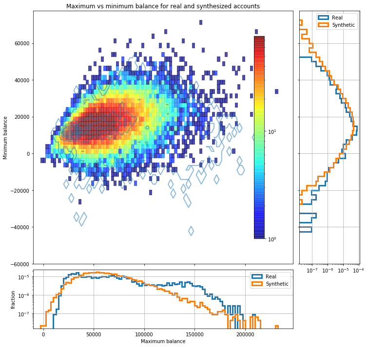
Regarding how well the global statistical properties of each account are reproduced, the following two plots show how the mean balance, standard deviation, minimum and maximum balance of each synthesized account are distributed compared with the same values for real accounts. In the main panel of each figure the 2D histogram corresponds to synthesized data whereas the contours correspond to real accounts.
Temporal aspects
Regarding the temporal aspects, it is analyzed how well the dates are synthesized with the encoding strategy. As mentioned before the date is decoded during post-processing using a start date, and the synthesized end of the month pseudo transactions and day of the month. The two following histograms compare globally the number of transactions per month and the time differences between two subsequent transactions in real and synthesized data.
The following figure shows the 2D histogram of average number of transaction per month in each account versus its standard deviation. It is observed that the synthesized transaction series behave well in this respect, even when few accounts present a high variation in the number of transactions per month that are not seen in the real data.
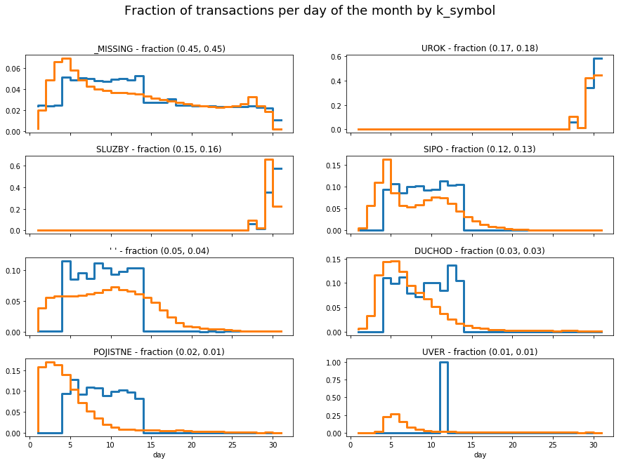
A final aspect to consider is how well the model reproduces when each transaction takes place. The following figures show the histograms of the day of the month for different type of transactions. The fraction of each type in the real and synthesized data is indicated in each panel. One can observe that, for the more frequent types the day is well reproduced whereas is not as well captured for less represented types.
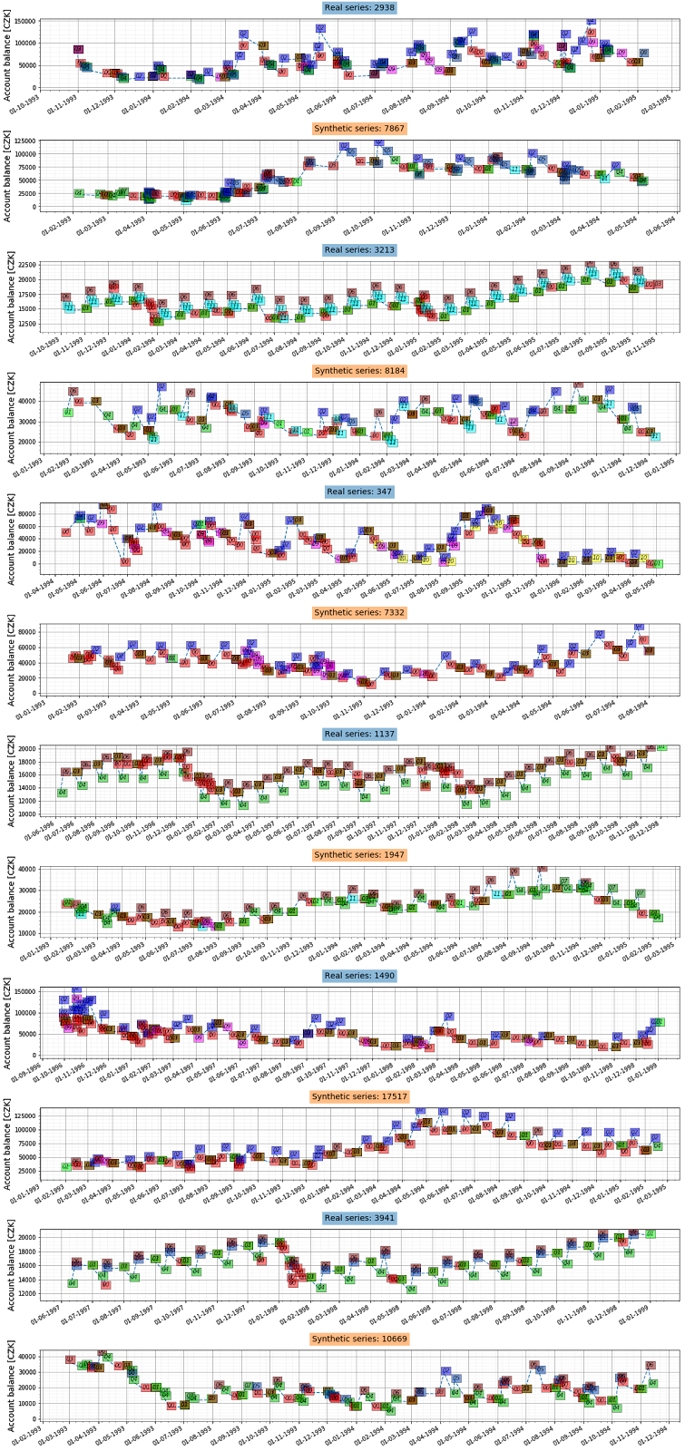
Finally, the next figures show some examples of real and synthesized transactions series. The y-axis displays the balance of the account after each operation. The colors indicate different types of transactions defined by the combination of (type, operation, and k_symbol).
Conclusions
The goal of this exercise was to test the potential of using a single deep neural network to synthesize complete series of banking transactions. This post illustrates the results: with the correct architecture and recurrent capacity it is possible to achieve a single model that performs well on the data used.
It is worth to mention that, in comparison with the data set used, present day bank transactions are significantly richer both in terms of information available for each entry, and in the frequency and the volume of operations. These factors may make the training of a single model more challenging. For example, a single model may fail to capture specific details that turn to be important. Modifying the training strategy to improve some aspects of the synthesis may have an unwanted effect in the model elsewhere. For these reasons, when working with more complex data sets, it can be beneficial to divide the system into components focused on reproducing the different dimensions of the data.
As a final comment, there are different circumstances that prevent the use or sharing of real data. In these situations, having systems with the capability of generating realistic data on demand can be crucial. Synthetic data can prove helpful in testing, software development, or even in the early stages of a machine learning solution. If you’re interested around any of the topics discussed, please check out the AI Team offering or contact us.
References